A Careful Control Loop
Sensor noise and uncertainty models is one lens on sensors, perception hardware, and state estimation. We study it because an embodied agent needs decisions that survive contact with noisy sensors, delayed effects, and changing environments.
This section develops the technical contract for Sensor noise and uncertainty models into a usable mental model. First we define the object of study, then we connect it to the agent loop, then we test it with a compact implementation.
The key question in Sensor noise and uncertainty models is practical: what must the agent know, what can it observe, what action is available, and what evidence shows that the action worked under the stated conditions?
A representation earns its place when it changes the measurable action interface. In Sensor noise and uncertainty models, the reader should keep asking which decision becomes easier, safer, or more reliable.
Theory
For Sensor noise and uncertainty models, the practical design rule is to make the interface inspectable before optimization begins: inputs, outputs, units, latency, bounds, and failure labels should all be visible in the saved artifact.
The mechanism in Sensor noise and uncertainty models is the contract between representation and action. Name what enters the module, what leaves it, which assumptions make that transformation valid, and which log would reveal a bad handoff.
Worked Example: Projecting a Point and Propagating Its Uncertainty
The right way to model a measurement is as a value plus a covariance. A 3D position estimate is a mean $X_w$ with a covariance $\Sigma_X$, and any function applied to that estimate transforms the covariance too. The pinhole camera is the canonical example. A world point projects to a pixel through the intrinsic matrix $K$ and the extrinsic pose $[R\,|\,t]$:
$$\lambda \begin{bmatrix} u \\ v \\ 1 \end{bmatrix} = K\,[R \mid t]\, X_w$$where $K$ holds the focal lengths and principal point, $[R\,|\,t]$ maps the world frame into the camera frame, and the scalar $\lambda$ is the point depth that is divided out to land on the image plane. Calibration is the process of recovering $K$ and the lens distortion from images of a known target. Because projection is nonlinear (the divide by depth), a 3D position uncertainty does not map to a simple fixed pixel uncertainty: depth error, in particular, blurs the pixel location more for nearby points. The example below projects one point and then propagates its 3D covariance to a pixel covariance by Monte Carlo, the same idea an extended Kalman filter would handle with a Jacobian.
# Project a 3D point to a pixel, then propagate its uncertainty to image space.
import numpy as np

K = np.array([[700.0,   0.0, 320.0],
              [  0.0, 700.0, 240.0],
              [  0.0,   0.0,   1.0]])
R = np.eye(3)                       # camera aligned with world axes
t = np.array([0.0, 0.0, 0.0])       # camera at the world origin
X_w = np.array([0.2, -0.1, 2.0])    # a 3D point, meters

Xc = R @ X_w + t                    # world -> camera frame
uvw = K @ Xc                        # apply intrinsics
u, v = uvw[0] / uvw[2], uvw[1] / uvw[2]   # divide by depth (lambda)
print(f"pixel = ({u:.1f}, {v:.1f})")

# 3D position uncertainty (depth noisier than lateral), propagated by sampling.
rng = np.random.default_rng(3)
Sigma_X = np.diag([0.01, 0.01, 0.04])     # variances in m^2
samples = rng.multivariate_normal(X_w, Sigma_X, size=5000)
proj = K @ samples.T
pix = (proj[:2] / proj[2]).T
print("pixel std (u, v):", np.round(pix.std(axis=0), 2))The fragment should compute one noise model, one residual, and one confidence interval. FilterPy, SciPy, and robot_localization scale that idea into maintained filters and diagnostics.
Practical Recipe
- Write the observation, action, and success metric before choosing a model.
- Build a baseline that is simple enough to debug by inspection.
- Add the library implementation only after the baseline behavior is understood.
- Record failures as structured cases: perception error, state error, planning error, control error, or evaluation error.
- Run at least one perturbation test before trusting the result.
The common mistake in Sensor noise and uncertainty models is to celebrate the component score before checking the closed-loop handoff. The failure usually appears at the boundary: stale state, wrong frame, delayed action, saturated actuator, or metric that ignores the real task cost.
A robotics team using Sensor noise and uncertainty models should log not only final success, but intermediate observations, chosen actions, controller status, and recovery events. The logs reveal whether the method is solving the task or merely passing the easiest episodes.
When sensor noise and uncertainty models feels abstract, ask what would be different in the next frame of video, the next robot state, or the next safety margin.
For Sensor noise and uncertainty models, treat frontier claims as hypotheses until they expose enough detail to reproduce the result: data boundary, embodiment, controller interface, evaluation panel, and failure cases.
Can you name the observation, state estimate, action, success metric, and most likely failure mode for Sensor noise and uncertainty models? If not, the system boundary is still too vague.
Production Pattern
Sensor noise and uncertainty models sits inside the Part II robotics contract: geometry defines where things are, kinematics defines what motion is possible, dynamics defines what motion costs, control defines how errors are corrected, and sensing defines what the agent can know on time.
Noise models should say what distribution is assumed, when it breaks, and how overconfidence is detected. This makes the section useful to students, builders, and researchers at the same time: the idea has an intuitive role, a formal interface, a runnable check, and a failure mode that can be reproduced.
For Sensor noise and uncertainty models, state estimation converts imperfect observations into a belief usable by control. Preserve calibration, covariance, timestamp, frame, dropout behavior, and latency.
| Tool or Library | What It Handles | Verification Check |
|---|---|---|
| OpenCV | handles camera models, calibration, projection, and vision preprocessing | Verify intrinsics, distortion, image timestamp, and frame-to-camera transform. |
| ROS 2 robot_localization | fuses odometry, IMU, GPS, pose, and twist streams through ROS estimation nodes | Verify covariance, frame IDs, timestamps, and rejected measurement counts. |
| FilterPy | teaches and prototypes Kalman, extended Kalman, unscented, and particle filters | Verify process noise, measurement noise, innovation, and covariance growth. |
| Kalibr | supports practical work on Sensor noise and uncertainty models | Verify the library output against the hand-built baseline on one small case. |
| Open3D | supports practical work on Sensor noise and uncertainty models | Verify the library output against the hand-built baseline on one small case. |
Use this recipe when turning Sensor noise and uncertainty models into code, a simulator experiment, or a robot diagnostic. The point is not to use every library. The point is to keep the hand-built baseline and the maintained-tool path comparable.
- Define each sensor message with units, frame, timestamp source, calibration file, and covariance meaning.
- Run a static test, a slow-motion test, and a dropout test before fusing streams.
- Compare the hand filter with FilterPy or ROS 2 robot_localization using identical measurements and noise settings.
- Log innovation, covariance, delayed messages, rejected measurements, and downstream control effect.
- Treat perception output as a belief with uncertainty, not as ground truth handed to the controller.
For Sensor noise and uncertainty models, compare methods only through one saved artifact that preserves the inputs, outputs, units, timestamps, latency budget, configuration, seed, metric definition, and failure labels relevant to this section. The comparison is meaningful only when the same script evaluates the same panel.
Extend the section exercise by adding one perturbation specific to Sensor noise and uncertainty models and one latency or uncertainty check. Save the result in the EvidenceRecord schema, then explain which library output you trust and why.
Uncertainty bugs masquerade as planning bugs when covariance is too small, non-Gaussian tails are ignored, or latency is treated as noise. Inspect residuals and confidence calibration before changing the controller.
Technical Core
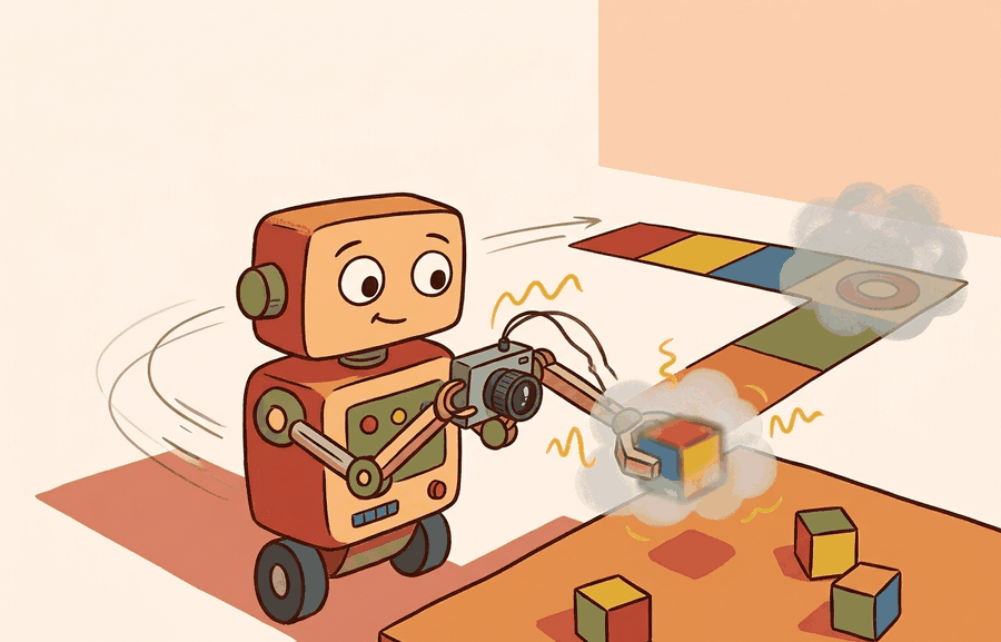
Sensor noise and uncertainty models explain how much trust a state estimator should place in each measurement. Noise is not only random scatter. Real sensors have bias, drift, quantization, dropout, saturation, outliers, and context-dependent error. Figure 8.5.T summarizes the chain this section must preserve when moving from a teaching example to a real embodied system.
The standard measurement model is $z_t=h(x_t)+v_t$ with $v_t\sim\mathcal N(0,R)$ when Gaussian noise is a reasonable approximation. Process uncertainty is usually written $x_t=f(x_{t-1},u_t)+w_t$ with $w_t\sim\mathcal N(0,Q)$. The matrices $R$ and $Q$ are not decorative tuning knobs: $R$ says how noisy the measurement is, while $Q$ says how wrong the motion model can be between measurements.
- Collect static data to estimate bias, variance, quantization, and dropout frequency.
- Collect controlled-motion data to separate sensor noise from motion-model error.
- Plot residuals and innovations before assuming they are Gaussian.
- Set $R$ from measured residual variance, then inflate it for context changes such as lighting, slip, vibration, or contact.
- Validate with normalized innovation squared, residual whiteness, and failure-labeled replay.
| Error Type | How It Appears | Diagnostic Check |
|---|---|---|
| Bias | Measurements are consistently shifted in one direction. | Static baseline and calibration target before and after operation. |
| Variance | Measurements scatter around the true value. | Residual histogram, covariance estimate, and innovation distribution. |
| Drift | Error grows slowly with time, temperature, or wear. | Long stationary run, warm-up comparison, and recalibration interval. |
| Outliers | Occasional measurements are far from the model. | Mahalanobis gating, robust residual plots, and raw-frame replay. |
| Dropout | Measurements disappear or arrive late. | Missing-data log, latency histogram, and estimator behavior during gaps. |
Expected output is an uncertainty model that predicts its own errors: roughly the right percentage of true states should fall inside the claimed confidence region. A tiny covariance with large innovations is an overconfidence bug, not a strong estimator.
A noise model fails when $R$ is copied from a datasheet, held constant across lighting or contact regimes, or tuned until the trajectory looks smooth while the innovation test is failing.
Section References
Core references for Sensor noise and uncertainty models: Modern Robotics; Murray, Li, and Sastry; Siciliano et al.; LaValle; and official documentation for Drake, MuJoCo, Pinocchio, CasADi, python-control, GTSAM, ROS 2, and OpenCV as applicable.
Use these references to check notation, frame conventions, units, solver assumptions, and maintained-library behavior.
Sensor noise and uncertainty models is useful when it makes the perception-action loop more reliable, not when it merely adds a more impressive model name.
Design a method-matched experiment for Sensor noise and uncertainty models. Specify the environment, observations, actions, metric, one perturbation, and the library output you would compare against the hand-built baseline.