The hardest part of driving is not seeing the world or steering the wheel; it is the handoff in between, where one subsystem's confident output becomes another's silent assumption.
On the architecture of the modern driving stack
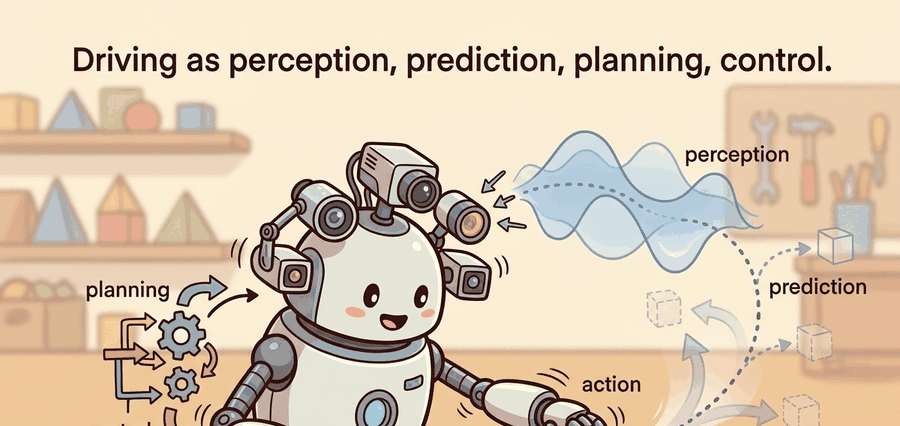
A modern autonomous vehicle is usually built as four cascaded subsystems: perception turns raw sensor streams into tracked objects and a drivable surface, prediction forecasts where dynamic agents will go, planning chooses a safe and comfortable trajectory, and control tracks that trajectory through the actuators. This section frames the whole vehicle as one closed loop so that the rest of the chapter can zoom into each stage without losing the interfaces that connect them.
This section develops driving as a closed loop rather than a label. The contract is concrete: ingest sensor streams, a map, and a route intent; estimate the state of the ego vehicle and of every relevant actor; commit to a trajectory; and convert that trajectory into steering, throttle, and brake commands at a fixed cycle rate. The loop is judged by route completion, collision rate, and safety margin, measured on the same scenarios for every candidate stack.
Real deployments run this loop at 10 to 20 Hz. A perception frame that arrives 150 ms late is not a slow frame; it is a wrong frame, because the planner will act on a world that has already moved. Treating the stack as a timed pipeline, not a static dataflow diagram, is the central discipline of the chapter.
The most instructive AV failures are not "the detector missed a pedestrian" but "the detector saw the pedestrian, the tracker dropped the track for two frames, and the planner therefore replanned through the gap." A perception improvement that never changes the planner's input does not reduce collisions. Always check whether an upstream win actually propagates to a downstream action.
Theory
Formally, driving is a partially observed Markov decision process run under hard real-time constraints. At cycle $t$ the vehicle receives an observation $o_t$ (camera frames, LiDAR sweeps, radar returns, GNSS or IMU), estimates a state $\hat s_t$ (ego pose and velocity plus a set of tracked actors with positions, velocities, and classes), commits to an action $a_t$ (a trajectory or a direct control command), and transitions to $o_{t+1}$. The decomposition into perception, prediction, planning, and control is an engineering factorization of this single MDP that makes each piece testable in isolation.
The factorization buys modularity at the cost of compounding error and interface mismatch. Perception errors (false negatives, identity switches, localization drift) become wrong inputs to prediction. Prediction errors (an unforecast lane change) become wrong inputs to planning. Each interface needs its own metric, and the whole stack needs a closed-loop metric, because passing every component benchmark does not guarantee a safe drive.
| Stage | Input | Output | Typical metric |
|---|---|---|---|
| Perception | raw sensor streams | tracked 3D objects, occupancy | mAP, MOTA, false-negative rate |
| Prediction | tracks plus map | multi-modal future trajectories | minADE, minFDE, miss rate |
| Planning | predictions plus route | ego trajectory | collision rate, comfort, progress |
| Control | ego trajectory | steer, throttle, brake | tracking error, jerk |
The loop is timed, not just connected. A common architecture runs perception and localization on a high-rate thread, prediction and planning on a slower deliberative thread, and a fast control thread that tracks the last committed trajectory until a new one arrives. A safety monitor watches the whole chain and triggers a minimal-risk maneuver (a controlled stop in lane or on the shoulder) when any subsystem stalls or disagrees beyond a threshold.
Worked Example
The example below is a minimal closed-loop simulation that exercises all four stages on a single car-following scenario. It exposes the interface fields a real stack must log: the estimated state, the prediction, the planned trajectory, and the control command, plus the safety margin that turns the run into evidence.
import numpy as np

# Ego and a lead vehicle on a straight road (1D for clarity).
ego = {"s": 0.0, "v": 12.0}        # position (m), speed (m/s)
lead = {"s": 30.0, "v": 8.0}       # slower lead vehicle ahead
dt = 0.1                            # 10 Hz control loop
T_HORIZON = 2.0                     # prediction/planning horizon (s)
TIME_GAP = 1.5                     # desired time gap (s)

def perceive(ego, lead):
    """Return measured gap and lead speed (noisy in reality)."""
    return lead["s"] - ego["s"], lead["v"]

def predict(gap, lead_v):
    """Constant-velocity forecast of the lead over the horizon."""
    return gap + (lead_v - ego["v"]) * T_HORIZON  # predicted future gap

def plan(gap, lead_v):
    """Choose target speed to hold a safe time gap (IDM-style)."""
    desired_gap = max(5.0, TIME_GAP * ego["v"])
    accel = 1.0 * (lead_v - ego["v"]) + 0.5 * (gap - desired_gap)
    return np.clip(accel, -4.0, 2.0)   # m/s^2, bounded actuator

def control(accel):
    """Convert planned acceleration into a (bounded) command."""
    return float(np.clip(accel, -4.0, 2.0))

for step in range(30):
    gap, lead_v = perceive(ego, lead)
    future_gap = predict(gap, lead_v)
    accel = plan(gap, lead_v)
    cmd = control(accel)
    # Apply control, advance the world one cycle.
    ego["v"] = max(0.0, ego["v"] + cmd * dt)
    ego["s"] += ego["v"] * dt
    lead["s"] += lead["v"] * dt
    if step % 10 == 0:
        print(f"t={step*dt:4.1f}s gap={gap:5.1f}m future_gap={future_gap:5.1f}m "
              f"v={ego['v']:4.1f} cmd={cmd:+.2f}")

print("min safety margin (gap) held:", round(lead['s'] - ego['s'], 2), "m")
Expected output: the gap shrinks from 30 m toward the desired time-gap distance and then stabilizes; the command saturates at the actuator limit during the initial deceleration and the final safety margin stays positive. The run is only useful as evidence because it logs the per-stage fields and the safety margin, not just "did not crash."
This hand-built loop shows the interfaces. For full experiments use a real simulator and middleware: CARLA and ROS 2 for closed-loop sensorimotor testing, nuScenes and the Waymo Open Dataset for logged perception and prediction, and a scenario runner for reproducible events. Keep the same artifact schema (per-stage logs plus a safety metric) whether you simulate by hand or in CARLA.
Practical Recipe
- Write the stack contract: the observation, the state estimate, the action interface, the cycle rate, and the safety metric.
- Build the smallest closed loop that can fail interpretably (the car-following example above).
- Add latency to one stage and measure how the safety margin degrades; this localizes timing brittleness.
- Replace one stage with the library version (for example a learned detector) and re-run on identical scenarios.
- Save one artifact: config, seeds, per-stage logs, summary metrics, and two representative traces (one nominal, one near-miss).
The classic mistake is to celebrate a component score before checking the handoff. A detector that improves mAP by feeding a richer object representation helps nothing if the prediction module only consumes bounding-box centers. Verify that each upstream improvement is actually read by the downstream consumer.
A robotics team integrating a new tracker should log intermediate tracks, predicted trajectories, the chosen plan, and every minimal-risk-maneuver trigger. When collision rate rises after the upgrade, those logs reveal whether the cause is more identity switches (perception), worse forecasts (prediction), or an over-conservative planner reacting to noisier tracks.
Perceive, predict, plan, control: four verbs, three interfaces, one loop. The bugs almost always live in the interfaces, not the verbs.
End-to-end and world-model driving (Sections 48.5 and the world-model material) challenge the four-box factorization by learning some or all of the stages jointly. The open question is whether a learned monolith can keep the per-stage observability that makes a modular stack debuggable and certifiable.
Can you name the observation, state estimate, action, success metric, and most likely failure mode for each of the four stages? If any cell is blank, the system boundary is still too vague to test.
| Tool or Library | Role in the Topic | Builder Advice |
|---|---|---|
| CARLA and ROS 2 | Closed-loop sensorimotor testing of the full stack | Adopt after the contract is explicit; keep one artifact schema across runs. |
| nuScenes, Waymo Open Dataset | Logged perception and prediction evaluation | Use for offline component metrics before closing the loop. |
| Same-panel evaluation script | Construct-matched stack comparison | Compare stacks only when collision rate and margin are co-computed on one scenario panel. |
Section 48.2 expands perception and sensor fusion, 48.3 covers detection and prediction, 48.4 and 48.8 cover planning, 48.7 covers control, and 48.6 and 48.9 close the loop with safety cases and closed-loop evaluation.
Take the car-following example, inject a one-cycle perception dropout (return the previous gap), and measure how much the minimum safety margin shrinks. Then label the failure as perception, state, planning, control, or timing.
Section References
Dosovitskiy et al., "CARLA: An Open Urban Driving Simulator," CoRL 2017. Caesar et al., "nuScenes: A Multimodal Dataset for Autonomous Driving," CVPR 2020. Sun et al., "Scalability in Perception for Autonomous Driving: Waymo Open Dataset," CVPR 2020.
These provide the simulator and benchmark datasets used to evaluate each stage and the closed loop.
Driving is one timed closed loop factored into four testable stages. The stack is only as reliable as its weakest interface, so every per-stage win must be verified to propagate all the way to the control command and the safety margin.
Design a same-panel experiment that swaps a constant-velocity predictor for a constant-acceleration predictor in the car-following loop. Specify the scenario set, the metric (minimum safety margin and collision rate), and the perturbation (a lead vehicle that brakes hard) that would reveal which predictor actually changes the control command.