A Careful Control Loop
Direct policy optimization trains the policy itself, not a value table that later chooses actions. Stochastic policies matter because an embodied robot must explore contact-rich behavior, represent uncertainty in perception, and keep a usable log probability for every action it took.
Value-based methods ask, "Which action has the highest estimated value?" Policy-gradient methods ask a different question: "How should the parameters of the action distribution move so future sampled behavior becomes more successful?" That shift is important in embodied control because the action may be continuous, multimodal, or constrained by hardware limits.
The object we optimize is the expected discounted return:
$$J(\theta)=\mathbb{E}_{\tau\sim\pi_\theta}\left[\sum_{t=0}^{T-1}\gamma^t r_t\right].$$
Here $\theta$ are policy parameters, $\tau$ is a trajectory of observations, actions, and rewards, $\pi_\theta(a_t \mid o_t)$ is the probability or density assigned to an action, and $\gamma$ discounts delayed consequences. Direct optimization means we adjust $\theta$ to increase $J(\theta)$ rather than first learning a separate action-value function and acting greedily from it.
A deterministic policy can only be judged by the action it already chose. A stochastic policy gives the learner a local experiment: it knows how probable the chosen action was, so it can increase that probability after good outcomes and decrease it after bad outcomes.
Theory
The policy is a distribution, not a lookup table. For a discrete mobile robot action set, $\pi_\theta$ might be a softmax over forward, left, right, and stop. For a manipulation controller, it might be a Gaussian over joint velocity commands with a learned mean and standard deviation. In both cases, the policy must expose two things for training: the sampled action and the log probability of that exact action.
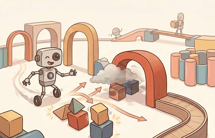
The central intuition is credit assignment through sampling. If a robot nudges a drawer handle and the drawer opens later, the update cannot differentiate through the drawer physics, contact impulses, camera exposure, or environment reset. It can still differentiate through the policy's own probability of the sampled motion. That is the foothold used by REINFORCE and PPO.
Direct policy optimization turns rollout data into pairs of log probabilities and returns. The update says, in effect, "actions that appeared in high-return trajectories should become more likely in similar observations, and actions from low-return trajectories should become less likely."
Worked Example
Code Fragment 1 below shows the smallest useful contrast: a deterministic controller always chooses the largest probability action, while a stochastic controller samples from the whole distribution and records the probability of what it did.
# Compare greedy action selection with stochastic sampling.
# The sampled action keeps a log probability, which policy gradients need.
import math
import random

random.seed(7)
actions = ["move_left", "move_right", "stop"]
logits = [0.2, 1.4, -0.7]

exp_logits = [math.exp(x) for x in logits]
total = sum(exp_logits)
probs = [x / total for x in exp_logits]

greedy_action = actions[probs.index(max(probs))]
sampled_action = random.choices(actions, weights=probs, k=1)[0]
sampled_prob = probs[actions.index(sampled_action)]

print("policy probabilities:", dict(zip(actions, [round(p, 3) for p in probs])))
print("greedy action:", greedy_action)
print("sampled action:", sampled_action, "log_prob:", round(math.log(sampled_prob), 3))move_left, move_right, and stop. The sampled action carries a log_prob, which is the training handle used later by REINFORCE and PPO.The worked example is small, but it shows the contract. The policy must not only choose an action; it must remember how surprising that action was under the current parameters. Without that record, the optimizer cannot say whether the action should become more or less likely after the return is known.
In practical experiments, Gymnasium provides the environment interface, and libraries such as CleanRL, Stable-Baselines3, RSL-RL, and rl_games keep the policy distribution, action sampling, and log-probability bookkeeping consistent. That does not remove the need to understand the contract; it keeps small bookkeeping errors from becoming training failures.
Practical Recipe
- Choose the policy distribution to match the actuator: categorical for discrete actions, Gaussian or squashed Gaussian for continuous commands.
- Log observations, sampled actions, rewards, terminations, and old log probabilities for every rollout step.
- Keep exploration physically plausible by bounding actions and standard deviations before the command reaches the controller.
- Evaluate with the same initial states and perturbations whenever two policy updates are compared.
- Separate policy failure from execution failure by logging controller saturation, contact slips, timeouts, and safety stops.
A policy can look stochastic in code while behaving deterministically in the robot. This happens when the action standard deviation collapses, action clipping hides large samples, or a low-level controller smooths every command into the same motion.
For a quadruped learning rough-terrain locomotion, a stochastic policy can try slightly different foot placements from the same body pose. The rollout log should preserve the sampled footstep command, its log probability, terrain patch features, slip events, and final stability score.
A stochastic policy is not indecisive. It is keeping receipts for the choices it made, so the optimizer can reward the useful experiments and retire the expensive ones.
Current embodied-policy research often combines stochastic policy gradients with demonstrations, offline datasets, safety filters, and diffusion-style action generators. The open question is how to preserve useful exploration while keeping real hardware inside safe contact, torque, and recovery limits.
For a robot arm policy, can you name the action distribution, the actuator bounds, the log-probability field saved in the rollout buffer, and the failure mode that would make the recorded probability misleading?
A direct policy optimizer only sees the consequences of actions that were actually sampled. That makes distribution design a systems decision, not a cosmetic modeling choice. Too little entropy prevents discovery; too much entropy spends rollouts on unsafe or uninformative behavior.
For embodied agents, the action distribution also sits between learning and control. A Gaussian policy over joint velocity commands may sample a value that the safety layer clips. If training records the unclipped log probability but the robot executes the clipped command, the update credits the wrong action. The implementation must log both the policy sample and the executed command.
| Action Space | Policy Form | Embodied Caution |
|---|---|---|
| Discrete mode choice | Categorical softmax | Make invalid actions impossible before sampling, not after the fact. |
| Joint velocity or torque | Gaussian with learned mean and scale | Track clipped commands because actuator limits change what the world receives. |
| Bounded continuous command | Tanh-squashed Gaussian | Account for the squashing transform when computing log probabilities. |
| High-level skill selection | Hierarchical categorical policy | Log the selected skill and the low-level controller outcome together. |
A robust implementation treats action sampling as part of the evidence artifact. Code Fragment 2 sketches the fields a rollout buffer needs before PPO or REINFORCE can make a valid policy-gradient update.
- Store the observation before action sampling, not a later state estimate after the controller has moved.
- Store the sampled action, executed action, old log probability, reward, value estimate, and termination flag in one row.
- Record the random seed and policy version that produced the rollout.
- Reject rollout rows where safety clipping or controller failure makes the training target ambiguous, or mark them with an explicit failure label.
- Compare policies only when rollouts use the same reset distribution and perturbation suite.
# Define the rollout row that direct policy optimization needs.
# Store both sampled and executed actions so safety clipping is visible.
from dataclasses import dataclass, asdict

@dataclass
class RolloutRow:
    observation_id: str
    sampled_action: float
    executed_action: float
    old_log_prob: float
    reward: float
    clipped_by_safety: bool

    def as_row(self) -> dict[str, object]:
        return asdict(self)

row = RolloutRow(
    observation_id="episode_0042_step_0017",
    sampled_action=1.35,
    executed_action=1.00,
    old_log_prob=-0.42,
    reward=0.8,
    clipped_by_safety=True,
)
print(row.as_row())RolloutRow separates sampled_action from executed_action. That distinction matters because policy-gradient math credits the sampled action, while the embodied system may have executed a clipped command.When direct policy optimization fails, first inspect the action distribution before blaming the optimizer. Check entropy, action clipping, invalid-action masking, controller saturation, and whether high-return episodes came from meaningful exploration or lucky resets. Then rerun a small perturbation panel with fixed seeds so the policy change is compared against the same embodied conditions.
For direct policy optimization, compare only construct-matched metrics co-computed in one pass on one configuration: same reset states, same policy checkpoint, same action bounds, same perturbation suite, and the same success definition. Save returns, action entropy, clipping rate, controller failures, and videos or state logs in one artifact so the policy improvement and the embodied behavior are backed by the same run.
Direct policy optimization works when the policy distribution, rollout buffer, and executed commands describe the same behavior. If those three records diverge, the gradient is learning from a story the robot did not actually enact.
Choose a discrete or continuous embodied task and write the policy distribution contract. Include the action bounds, sampling rule, log-probability field, safety clipping rule, and one diagnostic plot that would reveal exploration collapse.
What's Next?
This section established the policy distribution and rollout record that direct optimization needs. Next, Section 15.2 derives the likelihood-ratio estimator that turns those saved log probabilities into a policy-gradient update.
The original REINFORCE paper deriving the likelihood-ratio policy gradient. Read Section 2 for the REINFORCE update rule and Section 5 for baseline subtraction. This is the direct predecessor to actor-critic and PPO; understanding it makes the clipped surrogate objective in Schulman et al. 2017 concrete.
Formalizes the policy gradient theorem showing that the gradient of expected return can be expressed as an expectation over state-action pairs. Read to understand why on-policy sampling is sufficient for an unbiased gradient estimate and how the baseline reduces variance without introducing bias.
Schulman, J. et al. (2015). Trust Region Policy Optimization. ICML.
Introduces the trust-region constraint that bounds policy update size using KL divergence, providing a monotonic improvement guarantee. Read Section 3 for the surrogate objective and Theorem 1 for the lower bound; PPO simplifies this into a clipped ratio that achieves similar stability with far less implementation complexity.
Derives the generalized advantage estimator (GAE) as an exponentially weighted average of n-step returns, controlled by the lambda parameter. Read Section 3 for the bias-variance trade-off analysis; in practice lambda around 0.95 is the default in most PPO implementations and understanding why requires this paper.
Schulman, J. et al. (2017). Proximal Policy Optimization Algorithms. arXiv.
Introduces the clipped surrogate objective that prevents large policy updates without the second-order KL constraint of TRPO. Read Section 3 for the clipping mechanism and Section 5 for the implementation details including value-function loss coefficient and entropy bonus that appear in nearly every modern PPO codebase.
CleanRL documentation and source code.
Provides single-file, dependency-minimal RL implementations that make every algorithmic choice visible on one screen. Read the PPO and SAC files side by side with the corresponding papers; CleanRL is the fastest way to verify that you understand which implementation details matter versus which are optional.