A Careful Control Loop
Feedback, error, stability, overshoot, oscillation is one lens on Control for AI Practitioners. We study it because an embodied agent needs decisions that survive contact with noisy sensors, delayed effects, and changing environments.
This section develops the technical contract for Feedback, error, stability, overshoot, oscillation into a usable mental model. First we define the object of study, then we connect it to the agent loop, then we test it with a compact implementation.
The key question in Feedback, error, stability, overshoot, oscillation is practical: what must the agent know, what can it observe, what action is available, and what evidence shows that the action worked under the stated conditions?
A representation earns its place when it changes the measurable action interface. In Feedback, error, stability, overshoot, oscillation, the reader should keep asking which decision becomes easier, safer, or more reliable.
Theory
For Feedback, error, stability, overshoot, oscillation, the practical design rule is to make the interface inspectable before optimization begins: inputs, outputs, units, latency, bounds, and failure labels should all be visible in the saved artifact.
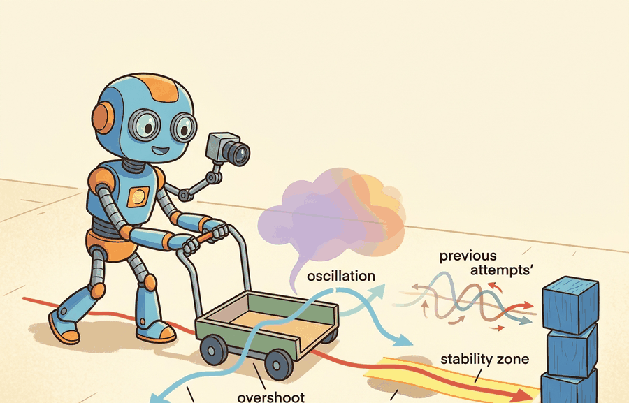
Feedback begins with an error signal, $e_t=r_t-y_t$, where $r_t$ is the reference and $y_t$ is the measured output. Stability asks whether a small disturbance stays bounded or shrinks; overshoot asks how far the response passes the target; oscillation asks whether correction arrives with the wrong phase or too much gain. For an AI practitioner, these are not abstract labels. They are log columns in a step-response test.
| Metric | What To Measure | What It Usually Means |
|---|---|---|
| Rise time | Time to move from near the start toward the target. | Low gain, heavy damping, or actuator limits can make the response slow. |
| Overshoot | Maximum amount past the target, often $(y_{\max}-r)/r$. | Feedback is aggressive relative to damping, delay, or mass. |
| Settling time | Time until the response remains inside a chosen tolerance band. | Residual oscillation, sensor noise, or weak damping keeps the loop busy. |
| Steady-state error | Final gap between target and measured output. | Bias, friction, gravity, or missing integral action is still present. |
The mechanism in Feedback, error, stability, overshoot, oscillation is the contract between representation and action. Name what enters the module, what leaves it, which assumptions make that transformation valid, and which log would reveal a bad handoff.
Worked Example
Stability of a linear system is decidable by inspection of one matrix. For \(\dot x = Ax\), the equilibrium is asymptotically stable exactly when every eigenvalue of \(A\) has a strictly negative real part. The Lyapunov view gives the same answer through an energy-like function: if there is a positive-definite \(P\) with \(\dot V(x) = x^\top(A^\top P + P A)x \le 0\), the system is stable. Code Fragment 7.2.1 takes a pendulum linearized near upright (an unstable plant), closes a PD loop around it, and verifies stability both ways.
import numpy as np
from scipy.linalg import solve_lyapunov

def classify(A):
    ev = np.linalg.eigvals(A)
    mx = np.max(ev.real)
    tag = "stable" if mx < 0 else ("marginal" if np.isclose(mx, 0) else "UNSTABLE")
    return ev, mx, tag

# Pendulum near upright: gravity term gives a positive eigenvalue -> it falls.
A_open = np.array([[0.0, 1.0],
                   [16.0, -0.2]])
# Proportional-derivative feedback u = -[k1 k2] x folded into the dynamics.
k1, k2 = 30.0, 8.0
A_cl = np.array([[0.0,        1.0],
                 [16.0 - k1, -0.2 - k2]])

for name, A in [("open-loop", A_open), ("PD closed-loop", A_cl)]:
    ev, mx, tag = classify(A)
    print(f"{name:>15}: eig = {np.round(ev, 3)}  max Re = {mx:+.3f}  -> {tag}")

# Lyapunov certificate for the stable loop: solve A^T P + P A = -Q, P must be PD.
Q = np.eye(2)
P = solve_lyapunov(A_cl.T, -Q)
print(f"Lyapunov P eigenvalues = {np.round(np.linalg.eigvalsh(P), 3)} (all > 0 proves stability)")The fragment should expose gain, pole location, settling time, overshoot, and oscillation. python-control makes the analysis repeatable, while logged step responses show whether the robot is stable in hardware.
Practical Recipe
- Write the observation, action, and success metric before choosing a model.
- Build a baseline that is simple enough to debug by inspection.
- Add the library implementation only after the baseline behavior is understood.
- Record failures as structured cases: perception error, state error, planning error, control error, or evaluation error.
- Run at least one perturbation test before trusting the result.
The common mistake in Feedback, error, stability, overshoot, oscillation is to celebrate the component score before checking the closed-loop handoff. The failure usually appears at the boundary: stale state, wrong frame, delayed action, saturated actuator, or metric that ignores the real task cost.
A robotics team using Feedback, error, stability, overshoot, oscillation should log not only final success, but intermediate observations, chosen actions, controller status, and recovery events. The logs reveal whether the method is solving the task or merely passing the easiest episodes.
Treat feedback, error, stability, overshoot, oscillation like a control-room label. If the label does not tell a future debugger what moved, what sensed, or what failed, it is decoration rather than engineering knowledge.
For Feedback, error, stability, overshoot, oscillation, treat frontier claims as hypotheses until they expose enough detail to reproduce the result: data boundary, embodiment, controller interface, evaluation panel, and failure cases.
Can you name the observation, state estimate, action, success metric, and most likely failure mode for Feedback, error, stability, overshoot, oscillation? If not, the system boundary is still too vague.
Production Pattern
Feedback, error, stability, overshoot, oscillation sits inside the Part II robotics contract: geometry defines where things are, kinematics defines what motion is possible, dynamics defines what motion costs, control defines how errors are corrected, and sensing defines what the agent can know on time.
Translate feedback behavior into measurable overshoot, settling time, steady-state error, and oscillation. This makes the section useful to students, builders, and researchers at the same time: the idea has an intuitive role, a formal interface, a runnable check, and a failure mode that can be reproduced.
For Feedback, error, stability, overshoot, oscillation, control closes the loop between estimated state and action. Keep reference, measured state, error signal, control law, actuator limits, and safety fallback separate in the evidence record.
| Tool or Library | What It Handles | Verification Check |
|---|---|---|
| python-control | analyzes linear systems, transfer functions, state-space models, and feedback loops | Verify units, sample time, poles, stability margin, and reference scaling. |
| CasADi | formulates optimization-based controllers with constraints and horizons | Verify constraints, warm start, solver status, and deadline behavior. |
| Drake | models dynamical systems, multibody plants, optimization, and controllers | Verify scalar type, plant finalization, frame convention, and solver status. |
| do-mpc | formulates optimization-based controllers with constraints and horizons | Verify constraints, warm start, solver status, and deadline behavior. |
| ROS 2 control | supports practical work on Feedback, error, stability, overshoot, oscillation | Verify the library output against the hand-built baseline on one small case. |
Use this recipe when turning Feedback, error, stability, overshoot, oscillation into code, a simulator experiment, or a robot diagnostic. The point is not to use every library. The point is to keep the hand-built baseline and the maintained-tool path comparable.
- Write the control objective, measured state, actuator command, update rate, and saturation policy.
- Run a step-response test before adding learning, with overshoot, settling time, and steady-state error logged.
- Compare the hand controller with python-control, CasADi, Drake, do-mpc, or ROS 2 control on the same plant model.
- Record latency, missed deadlines, saturation events, constraint violations, and recovery actions.
- Only compare controllers and policies when they share sensors, action limits, disturbance tests, and safety checks.
For Feedback, error, stability, overshoot, oscillation, compare methods only through one saved artifact that preserves the inputs, outputs, units, timestamps, latency budget, configuration, seed, metric definition, and failure labels relevant to this section. The comparison is meaningful only when the same script evaluates the same panel.
Extend the section exercise by adding one perturbation specific to Feedback, error, stability, overshoot, oscillation and one latency or uncertainty check. Save the result in the EvidenceRecord schema, then explain which library output you trust and why.
A learned policy can hide an unstable inner loop until the disturbance changes. Check update rate, delay, saturation, integral windup, and fallback behavior before scaling training. For this section, first reproduce one tiny step response by hand, then rerun it through python-control, CasADi, Drake, do-mpc, or ROS 2 control. If the two disagree, inspect sample time, sign convention, measurement delay, and output units before changing the model.
Technical Core
Feedback, error, stability, overshoot, oscillation needs a topic-native core: variables, equations or system contracts, an algorithmic procedure, an expected output, and a failure diagnosis. Figure 7.2.T summarizes the chain this section must preserve when moving from a teaching example to a real embodied system.
Error is $e_t=r_t-y_t$. Overshoot for a positive step can be recorded as $M_p=(y_{\max}-r)/|r|$. A discrete loop is practically stable when bounded perturbations produce bounded, decaying deviations under the same sample time, actuator limits, and sensor delay used in deployment.
- Define the reference, measured state, error signal, actuator command, update rate, and saturation policy.
- Run a step or disturbance response before adding learning.
- Log overshoot, settling time, steady-state error, latency, saturation, and recovery behavior.
- Compare PID, LQR, or MPC only under the same plant, sensors, limits, disturbance panel, and metric code.
| Contract Field | What To Specify | Why It Matters |
|---|---|---|
| State and observation | Variables, units, timestamps, frames, and uncertainty. | Prevents a model score from being mistaken for robot capability. |
| Action interface | Command type, limits, update rate, and safety fallback. | Makes the learned or planned output executable. |
| Evidence artifact | Trace, metric, configuration, seed, and failure label. | Allows baseline and library path to be compared in one pass. |
| Tool path | python-control, CasADi, do-mpc, Drake, ROS 2 control, MuJoCo | Shows the practical library route after the mechanism is understood. |
For Feedback, error, stability, overshoot, oscillation, expected output is a trace where the relevant error decreases, overshoot stays within the design bound, and actuator commands remain within limits under the stated timing budget.
Feedback, error, stability, overshoot, oscillation should be stress-tested under delay, integral windup, actuator saturation, unmodeled friction, and reference-frame mismatch before the nominal trace is trusted.
Section References
Core references for Feedback, error, stability, overshoot, oscillation: Modern Robotics; Murray, Li, and Sastry; Siciliano et al.; LaValle; and official documentation for Drake, MuJoCo, Pinocchio, CasADi, python-control, GTSAM, ROS 2, and OpenCV as applicable.
Use these references to check notation, frame conventions, units, solver assumptions, and maintained-library behavior.
Feedback, error, stability, overshoot, oscillation is useful when it makes the perception-action loop more reliable, not when it merely adds a more impressive model name.
Design a method-matched experiment for Feedback, error, stability, overshoot, oscillation. Specify the environment, observations, actions, metric, one perturbation, and the library output you would compare against the hand-built baseline.