For Robustness and generalization metrics, a benchmark conclusion survives reruns only when the panel, seed policy, exclusion rules, and raw episode artifacts are inspectable.
An Evaluation Methodologist
Nominal average return is only one slice of evaluation. Embodied systems also need shift-sensitive, worst-case, and outlier-aware metrics because the world does not sample only clean conditions.
Why This Matters
Robustness and generalization metrics matters because evaluation choices rewrite the scientific claim. If the metric drops time, energy, or safety terms that the deployment team cares about, the benchmark no longer matches the real decision.
A compact robustness report can include the clean score $J_{clean}$, the mean shifted score $J_{shift}$, and the tail-risk statistic $$\text{CVaR}_{\alpha}(L) = \mathbb{E}[L \mid L \ge q_{\alpha}],$$ where $L$ is loss and $q_{\alpha}$ is the upper-tail quantile. This keeps average and worst-case behavior visible together.
Generalization is not a single number. It has at least three faces: interpolation to new task instances, robustness to nuisance perturbations, and behavior under truly out-of-support states.
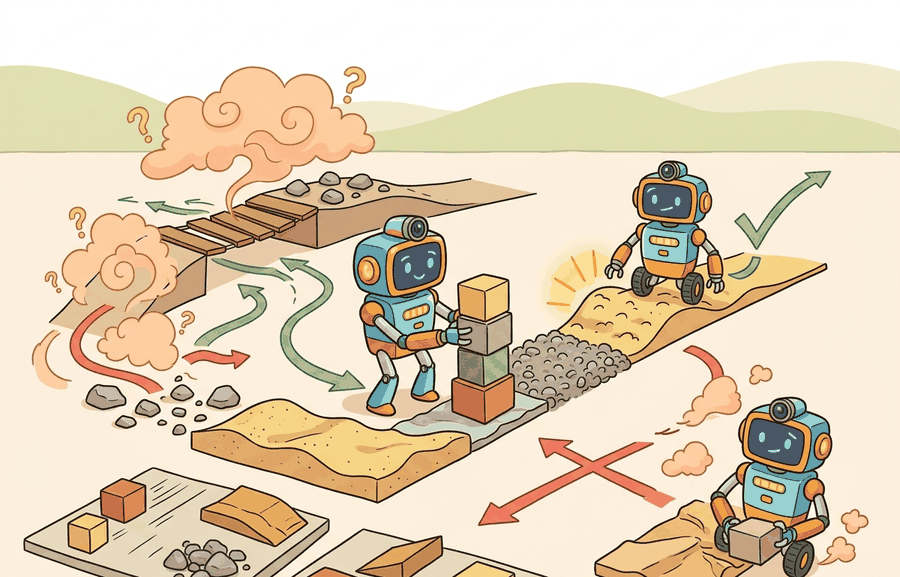
- Partition the rollout panel into clean, interpolated, shifted, and stress-test slices.
- Compute average performance on each slice and a tail-risk statistic on the hardest slice.
- Report confidence intervals per slice, not only globally.
- Store enough metadata to recreate which perturbation family produced each tail event.
- Rank models only after checking whether one model's gain is just a clean-slice artifact.
Worked Example
Two drone policies can tie on average mission success while differing dramatically on gust-heavy scenes. The difference may only appear in the worst decile of episodes, which is why tail metrics matter.
losses = [0.1, 0.2, 0.25, 0.3, 0.35, 0.9, 1.1, 1.4]
alpha = 0.75
threshold_index = int(alpha * len(losses))
q_alpha = sorted(losses)[threshold_index]
tail = [x for x in losses if x >= q_alpha]
cvar = sum(tail) / len(tail)
print({"q_alpha": q_alpha, "cvar": round(cvar, 3), "tail_count": len(tail)})
{'q_alpha': 0.9, 'cvar': 1.133, 'tail_count': 3}Expected output: The output identifies the tail threshold and the mean of the worst episodes. A large gap between average loss and CVaR signals brittle behavior hidden by nominal aggregates.
Use a dataframe pipeline plus SciPy or NumPy quantile utilities for production analysis. The important part is not the software, but that clean, shifted, and tail slices are all computed from the same stored episodes.
Robustness and generalization require stratified panels rather than one pooled score. Pandas separates lighting, geometry, payload, terrain, object, and operator factors; SciPy evaluates paired deltas inside each stratum; DVC freezes the panel; and ROS 2 bags keep the physical context for every out-of-distribution claim.
Embodied robustness work benefits from treating perturbation families as experimental factors. Lighting shift, texture shift, actuation delay, and friction change should each have their own slice before they are rolled into an aggregate robustness view.
The useful artifact here is a generalization matrix whose rows are perturbation families and whose columns are task success, constraint margin, latency, and recovery. It prevents interpolation wins from being confused with true operating-envelope expansion.
A common benchmark error is to mix interpolation and true OOD states into one bucket called generalization. That makes it impossible to tell whether the model fails because of modest novelty or because the state is physically outside the training support.
Cross-References
This section prepares the ground for Section 53.1 on disturbance classes and Section 53.3 on OOD detection.
Take one existing evaluation table and split it into clean, shifted, and stress-test slices. Add a CVaR column and compare whether the method ranking changes.
Do not declare a model robust because it survived one handpicked perturbation family. Robustness claims require coverage across perturbation classes and disclosure of where the model remains weak.
For a humanoid locomotion controller, clean floors, mild friction changes, and severe friction drops should appear as separate rows. The right policy may be worse on average but far safer in the tail.
Current research is moving toward richer perturbation taxonomies, compositional shift panels, and benchmark artifacts that keep the perturbation generator itself versioned and auditable.
Can you distinguish the average shifted score from a tail-risk statistic like CVaR? If not, your robustness vocabulary is still too coarse.
Generalization metrics should preserve clean, shifted, and worst-case structure. One average score is rarely enough for embodied deployment decisions.
Define a robustness report for one robot task with at least three perturbation families and one tail metric. Explain which deployment question each slice answers.
A policy that gets 90 percent on clean scenes and 12 percent in rain is not a robustness story. It is a weather forecast with expensive consequences.
Section References
Ovadia, Y. et al. "Can You Trust Your Model’s Uncertainty? Evaluating Predictive Uncertainty Under Dataset Shift." (2019). https://arxiv.org/abs/1906.02530
A helpful bridge between shift evaluation and calibrated uncertainty.
Agarwal, R. et al. "Deep Reinforcement Learning at the Edge of the Statistical Precipice." (2021). https://arxiv.org/abs/2108.13264
Useful for careful metric aggregation and confidence intervals.
Section 52.5 now asks when simulation can stand in for physical evaluation and what evidence is needed to justify that proxy.